Procedural Generation with Wave Function Collapse

(Edit 2022-05-03: I found out that the Wave Function Collapse algorithm was heavily inspired by an existing algorithm called “Model Synthesis”. I’ve added a section to further reading with links to the author’s website for more information.)
Wave Function Collapse is a procedural generation algorithm which produces images by arranging a collection of tiles according to rules about which tiles may be adjacent to each other tile, and relatively how frequently each tile should appear. The algorithm maintains, for each pixel of the output image, a probability distribution of the tiles which may be placed there. It repeatedly chooses a pixel to “collapse” - choosing a tile to use for that pixel based on its distribution. WFC gets its name from quantum physics.
The goal of this post is to build an intuition for how and why the WFC algorithm works.
I will break WFC into two separate algorithms and explain them separately. Each is interesting in its own right, and the interface between them is simple.
Core Interface
fn wfc_core(
    adjacency_rules: AdjacencyRules,
    frequency_rules: FrequencyHints,
    output_size: (u32, u32),
) -> Grid2D<TileIndex> { ... }
This is the low-level part of the algorithm which solves the problem of arranging tiles into a grid according to some specified rules. I’ll give a “black box” description of the core here, and explain how it works internally below.
Adjacency Rules
The “core” receives a set of adjacency rules describing which tiles may appear next to other tiles in each cardinal direction. Some example rules are “Tile 6 may appear in the cell ABOVE a cell containing tile 4”, and “Tile 7 map appear in the cell to the LEFT of a cell containing tile 3.
Frequency Hints
It also receives a set of frequency hints, which is a mapping from each tile to a number indicating how frequently the tile should appear in the output, relative to other tiles. If tile 4 maps to 6, and tile 5 maps to 2, then tile 4 should appear 3 times as frequently than tile 5.
Tile Index
The core doesn’t actually get to see the tiles themselves. Rather, tiles are referred to by integers ranging from 0 to the number of tiles minus 1, which I’ll refer to as tile indices. The adjacency rules and frequency hints are all specified in terms of tile index.
Output
The algorithm populates a grid with tile indices in a way which completely respects adjacency rules, and probabilistically respects frequency hints. Every pair of adjacent tiles will be explicitly allowed by the adjacency rules, and the relative frequencies of tiles in the output will usually be about the same as in the frequency hints.
Image Processor
This is the “glue” between the core algorithm, and an input and output image. Typically WFC is used to generate output images which are “similar” to input images. There’s no requirement that the output image be the same dimensions as the input image. Specifically, similar means that for some tile size:
- every tile-sized square of pixels in the output image appears somewhere in the input image
- the relative frequencies of tile-sized squares of pixels in the output image is roughly the same as in the input image
In other words, the output image will have the same local features as the input image, but the global structure may be different.
Note that there are some alternative applications of WFC besides generating similar images, such as arranging hand-crafted tiles with user-specified adjacency rules and frequency hints. These applications would still use the same core algorithm, but the image processor would be different.
Pre Processing
fn wfc_pre_process_image(
    input_image: Image,
    tile_size: u32,     /* often 2 or 3 */
) -> (AdjacencyRules, FrequencyHints, HashMap<TileIndex, Colour>) { ... }
The goal of this step is to generate adjacency rules and frequency hints which will be passed as input to the core algorithm.
First, we need to know what the different tiles are. Given an input image and tile size, enumerate all the tile-sized squares of pixels from the input image, including those squares whose top-left pixel occurs within tile size of the right and bottom edges, wrapping around to the other side of the input image in such cases.
Consider this 4x4 pixel input image:

With a tile size of 3, the first 3 tiles created by looking at squares of pixels with their top-left corners along the top row of pixels:


In the 3rd tile, we sampled off the edge of the image. In such cases, wrap around to the other side of the image. Effectively pretend that the image repeats forever in all directions.
Continuing in this fashion, enumerate all the tiles. In this example there are 16, and all are unique.
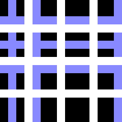
Assign each tile a tile index. In the example, we would use numbers from 0 to 15 as indices. Frequency hints and adjacency rules will be given in terms of tile indices, rather than tiles themselves.
The next few sections will explain how to construct frequency hints and adjacency rules so the core algorithm generates images which are similar to the input.
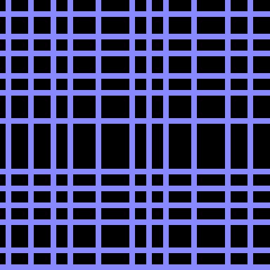
Here’s an image which is similar to the example image, generated using WFC:
Reflection and Rotation
When generating tiles from an input image, you may want to include tiles which aren’t necessarily present in the input image, but which are the rotation or reflection of tiles from the input image.
We need a new example image to demonstrate this, as each rotation and reflection of each tile is also in the tile set. Let’s use the following input image:

With a tile size of 3, the top-left tile we extract will be:

All rotations and reflections of this tile:


Repeat this for all the tiles extracted from the image.
To include these tiles in the output, proceed with the rest of the algorithm as normal, with these added to the tile set as fully qualified tiles, with their own unique tile indices.
A similar image to the input without rotations or reflections included:
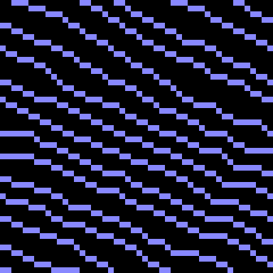
Here’s an output with all rotations and reflections included:
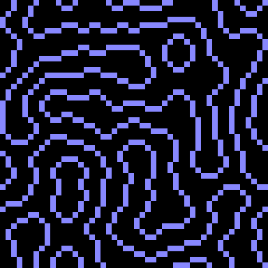
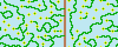
The banner at the top of this page was generated from the following image including all rotations and reflections:

Here’s a miniature version:
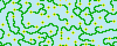
Notice that the ground is missing? Since the input image is wrapped, there are no tiles in which the ground ends or changes direction. This means that if the ground is present in the output, it must form a solid line from one side of the output to the other. This is a fairly restrictive constraint, so in most output, there is no ground at all. It’s possible for the output to deviate from the frequency hints if the structure of the image means there is no way to place a tile without violating the adjacency rules.
There is a small chance of the output containing ground:
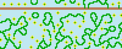
It’s not on the bottom of the screen, because the input image is wrapped.
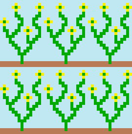
Since this was generated with rotations and reflections included, there’s nothing to stop the ground from being vertical.
Frequency Hints
The number of occurrences of each tile in the input image is counted, and mappings from a tile’s index to its count make up the frequency hints.
Let’s modify the first example image:

The set of unique 3x3 tiles in this input image will be the same as the first example, however where in the first example each tile appeared exactly once, here some patterns appear several times.
The following tiles appear 5 times in this image:


The remaining tiles still just appear once.
The relative frequency the above 4 tiles will be 5, and the hint for the other tiles will be 1. This means that the above 4 tiles are 5 times as likely to appear in a given position as the other tiles.
How do you think this will change the output?
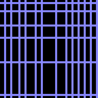
Increasing the odds of vertical lines appearing means there will likely be more vertical lines. This manifests as the grid cells in the image generally being taller than they are wide.
Adjacency Rules
The core will produce a grid of tile indices where each index corresponds to a single pixel in the output image. For a given tile index in a cell of this grid, the output pixel corresponding to the cell, will be given the colour of the tile corresponding to the tile index. Only the colour of the top-left pixel of the tile will be used. Keep that in mind for this section: for every tile placed, only a single pixel of the tile (its top-left pixel) is actually added to the output image. As the core assigns pixel indices to grid cells, we can say that the core assigns the top-left corners of tiles to output image pixels.
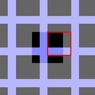
Remember that the goal of the image processor is to produce an output image where every tile-sized square of pixels occurs in the input image. In order to meet this goal, we must ensure that whenever the core assigns the top-left pixel of a tile to a pixel of the output image, the rest of the pixels of the tile end up in the right places as well. This is best explained with an example. Here’s a zoomed-in section of the banner:
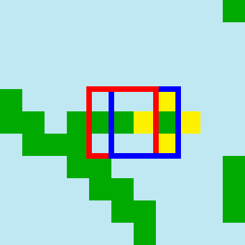
Consider the 3x3 pixel square with a red border. It occurs in the input image (rotated anticlockwise 90 degrees, below the bottom-right flower). Let’s assume it gets tile index 7. The core algorithm decided that the grid cell corresponding to the top-left pixel in the red square, should contain tile index 7. Even though tile index 7 refers to the whole 3x3 tile (but only the image processor knows this), choosing tile index 7 for this cell resulted in only the top-left pixel of the output image being populated.
But somehow the rest of the red square ended up looking like the tile with tile index 7 as well. But why? Every time a tile index is assigned to a cell, we want a way to make sure that the entire tile’s pixels - not just its top-left pixel - end up in the right output pixels, relative to the tile’s placement. Since each tile placement just contributes the tile’s top-left pixel, we need to make sure that whenever a tile is placed within tile size pixels of an already-placed tile’s top-left pixel, that the newly placed tile’s pixels don’t conflict with the pixels of the already-placed tile.
A convenient fiction to help picture this, is to imagine that whenever the core places a tile in a cell, each pixel in the tile-sized square of pixels whose top-left corner is that cell, is coloured to match the corresponding pixel of the tile, but only the top-left cell is marked as “populated”. Unpopulated (but possibly coloured) cells can have tiles placed in them, as long as all cells in the square filled by the new tile are either not yet coloured, or contain the same colour as the corresponding pixel of the new tile.
Let’s generate adjacency rules to force the core to never place two tiles in positions where their overlapping pixels conflict. Recall that an adjacency rule is of the form: “Tile index A may appear in the cell 1 space in DIRECTION from a cell containing tile index B”. The rules should only permit A to be placed adjacent to B in DIRECTION if doing so would not cause a conflict. All non-conflicting adjacencies should be allowed.
let mut adjacency_rules = AdjacencyRules::new();
for a in all_tiles {
    for b in all_tiles {
        for direction in [LEFT, RIGHT, UP, DOWN] {
            if compatible(a, b, direction) {
                adjacency_rules.allow(a, b, direction);
            }
        }
    }
}
The compatible(a: Tile, b: Tile, direction: Direction) -> bool function returns true if and only if overlapping
a with b, if b is offset by 1 pixel in direction, the overlapping parts
of the two tiles are identical.
In the example below, compatible(A, B, RIGHT) == true.
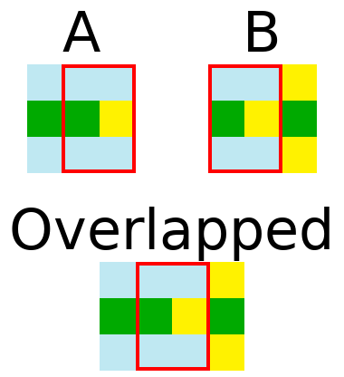
In this example tiles are 3x3, but these adjacency rules only ensure that adjacent tiles are compatible. It’s possible for a pair of tiles which are 2 pixels apart to overlap. What prevents them from conflicting?
Consider this example:
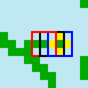
The red and blue squares surround tile placements which are 2 pixels apart. They aren’t adjacent, so the adjacency rules don’t explicitly forbid the red tile’s pixels and blue tile’s pixels from being different in the intersecting area.
However, the existence of the black square, which is adjacent to both the red and blue squares, means that the red and blue tile placements won’t conflict.
Because they are adjacent, the red/black intersection and the blue/black intersection are conflict-free. That is, the colours of pixels in the intersecting parts of the tiles are the same in both tiles. Red/blue is contained in both red/black and blue/black. Since the pixel colours in the red/blue region of red are the same as the pixel colours in the corresponding region of black, and the pixel colours in the red/blue region of black are the same as the pixel colours in the corresponding region of blue, the pixel colours in the red/blue region of red are the same is the pixel colours of the corresponding region of blue. That is, red/blue is conflict free.
Tile/Colour Mappings
After preprocessing, the frequency hints and adjacency rules will be passed to the core algorithm, and it will return a grid of tile indices. To produce the output image, we will need to know which tile index refers to which colour. To help with this, the preprocessor outputs a map from tile index to the colour of the top-left pixel of the corresponding tile.
Post Processing
fn wfc_post_process_image(
    tile_index_grid: Grid2D<TileIndex>,
    top_left_pixel_of_each_tile: HashMap<TileIndex, Colour>,
) -> Image { ... }
The final step is trivial. Take the grid of tile indices produced by running the core algorithm on the adjacency rules and frequency hints from the preprocessor, and the top-left pixel colour map, also returned by the preprocessor, and create an output image of the same dimensions as the grid. For each tile index in the grid, set the corresponding pixel colour in the output image to be the colour associated with that tile index in the top-left pixel colour map.
Putting it all together
Composing these pieces gives the full WFC algorithm.
fn wfc_image(image: Image, tile_size: u32, output_size: (u32, u32)) -> Image {
    let (adjacency_rules, frequency_hints, top_left_pixel_of_each_tile) =
        wfc_pre_process_image(image, tile_size);
    let tile_index_grid = wfc_core(adjacency_rules, frequency_hints, output_size);
    return wfc_post_process_image(tile_index_grid, top_left_pixel_of_each_tile);
}
Core Internals
My goal for this section is to impart a deep understanding of how and why the core algorithm works. This is the guide I wish I had during my implementation of WFC. Maybe it can help you through yours!
Sudoku
Imagine you’re solving a sudoku.
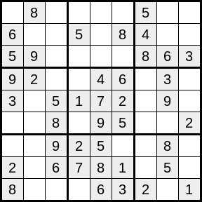
Your goal is to place a number from 1-9 in each empty cell, such that each row, column, and 3x3 square, contains each number from 1-9 exactly once.
Suppose you’re not super-confident in your sudoku-solving abilities, and your pencil comes equipped with an eraser. You could cheat, by writing in each cell (in tiny writing) all the possible values for that cell. Once all the cells are enumerated in this fashion, hopefully there will be some cells with a single possible value. For each of these cells, you erase the tiny pencil number, and rewrite the number in permanent marker, “locking in” your solution for that cell.
After locking in a cell, you want to update your enumerated possibilities for other cells in the same row, column, and 3x3 square, erasing all instances of the number you just locked in. You hope that by doing this, you’ll eliminate enough possibilities that the next choice becomes obvious, and so on until you’ve solved the entire sudoku in the least fun way possible! (This algorithm doesn’t actually work in all cases, so you may occasionally have to employ some actual thought!)
Now, imagine you wanted to solve an empty sudoku in the same way as just described:
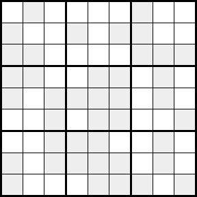
Your goal is still to end up with the numbers from 1-9 in every row, column, and 3x3, but this time you’re searching for one of a large number of possible solutions. You start by writing in tiny pencil digits, the numbers from 1-9 in each cell. Now you have a conundrum! Which cell do you lock in first? What number to you write first?
Say you make your first choice arbitrarily, and write a big 3 in pen in the top-left corner. Now you can propagate the effect of this choice by scanning along the top-most row, left-most column, and top-left 3x3 square, and erasing all the 3s.
What next?
If you keep choosing arbitrarily, it’s very likely that at some point, you’ll lock in a number, propagate the effect, and end up erasing the last penciled-in number in a cell. That would be bad, as then there would be no way to complete the soduku!
Maybe you’re ok with screwing up occasionally, as long as there’s a reasonable chance that you’ll end up with a valid solution each time. Then if you get into a bad state (ie. a cell with no possibilities), you can just give up and start over.
Intuitively, when choosing which cell to lock in next, you might want to always choose the cell with the fewest remaining possibilities. If there are several cells tied for the fewest remaining possibilities, choose arbitrarily between them.
Concretely, your strategy is to repeat the following until all cells are locked in:
- Choose a cell at random, considering only the cells with the fewest possible values.
- Choose a random value to lock in for that cell, considering only the possible values for that cell.
- Propagate the effects of locking in the cell, removing the locked-in value from the possibilities of cells sharing the cell’s row, column, and 3x3 square.
- If during propagation, you removed the final possibility of a cell, give up and start again.
The core WFC algorithm looks very similar to this. In place of the rules of sudoku, there are the adjacency rules. The frequency hints mean that when choosing a value to lock in, you no longer make a uniformly random choice, but instead choose from a probability distribution of the possible tile indices, weighted by frequency hints. The fact that some tiles are more likely to appear than others means the choice of which cell to lock in next is a little more complicated than just choosing from the cells with the fewest possibilities. Finally, we’re going to be more clever about propagation than in the sudoku example; you don’t have to wait until a cell is locked in to eliminate possibilities from surrounding cells.
Rough Sketch
Here’s a rough outline of the types and methods that the core will use. I’ll fill in details as they become relevant. In the spirit of Wave Function Collapse, “collapsing” a cell will refer to locking-in the choice of which tile index will go in the cell.
// Tile indices are just integers
type TileIndex = usize;

// corresponds to a cell in the output grid
struct CoreCell {
    // possible[tile_index] == true means tile_index may be chosen for this cell.
    // Initially, every element of this vector is `true`.
    // There is one element for each unique tile index.
    possible: Vec<bool>,
    ...
}

struct CoreState {
    // corresponds to the output grid
    grid: Grid2D<CoreCell>,
    // initialised to the number of cells in `grid`
    remaining_uncollapsed_cells: usize,
    // arguments passed from image processor
    adjacency_rules: AdjacencyRules,
    frequency_hints: FrequencyHints,
    ...
}

impl CoreState {

    // return the coordinate of the next cell to collapse
    fn choose_next_cell(&self) -> Coord2D { ... }

    // collapse the cell at a given coordinate
    fn collapse_cell_at(&mut self, coord: Coord2D) { ... }

    // remove possibilities based on collapsed cell
    fn propagate(&mut self) { ... }

    // roughly the same as the empty sudoku solver
    fn run(&mut self) {
        while self.remaining_uncollapsed_cells > 0 {
            let next_coord = self.choose_next_cell();
            self.collapse_cell_at(next_coord);
            self.propagate();
            self.remaining_uncollapsed_cells -= 1;
        }
    }
}
The remainder of this chapter will flesh out the details of choose_next_cell,
collapse_cell_at, and propagate.
Choosing the Next Cell to Collapse
In the sudoku example, we just chose randomly between the cells with the fewest
valid choices, to reduce the odds of removing all possibilities from a cell.
The intuition behind this is to lock in one of the cells with the
least uncertainty. In information theory, this uncertainty is known as
entropy. The goal
of this step is to choose randomly between the cells whose entropy is lowest.
The possible field of CoreCell can tell us which tiles are allowed in a
given cell, and the FrequencyHints can tell us how likely a given tile is to
appear in any cell.
Entropy Primer
If you have an unknown value with n possibilities: x1, x2, …, xn,
and the probability of a given value x, represented as a number between 0 and 1, is expressed as P(x), then the
entropy of your unknown value is:
- P(x1)*log(P(x1)) - P(x2)*log(P(x2)) - ... - P(xn)*log(P(xn))
…where the base of the logarithm is arbitrary. Let’s use 2 as our base.
To help build an intuition for this, first note that P(x) for all
possibilities will be between 0 and 1, and the sum:
P(x1) + P(x2) + ... + P(xn)
…is equal to 1. This is because x1…xn covers all possible outcomes, and one of the
outcomes will end up happening.
Each term in the entropy equation is negated. This is because P(x) is between
0 and 1, and regardless of the base, the logarithm of values between (exclusive)
0 and 1 is negative. Here’s a graph of log base 2:
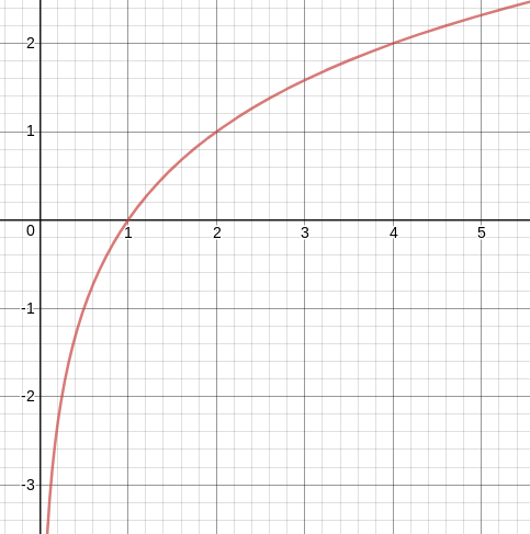
Since each term contains log(P(x)), which is always negative, we negate each
term to make the resulting entropy positive, as otherwise it would always be
negative.
A special case
We can simplify the entropy equation for the purposes of this algorithm.
If you have an unknown value with n possibilities: x1, x2, …, xn,
and each probability P(x) can be represented by w1 / (w1 + w2 + ... + wn)
(w stands for “weight”), then the above entropy equation can be simplified.
In practical terms, this is the case when you have a discrete probability
distribution - that is, you associate a weight wk with each possibility xk.
The probability of an outcome is its weight divided by the sum of all weights.
Let W = w1 + w2 + ... + wn be the sum of all weights.
Then the entropy of the unknown value is:
log(W) - (w1*log(w1) + w2*log(w2) + ... + wn*log(wn)) / W
You can derive this equation from the original entropy equation and log identities. It’s very satisfying. Try it!
Relative Tile Frequencies
This simplified entropy definition is relevant to choosing the next cell, as the frequency hint is effectively a discrete probability distribution of possible choices of tile.
Let’s declare some methods of FrequencyHints and CoreCell:
impl FrequencyHints {
    // Returns the number of times the corresponding tile appears in the input.
    // This corresponds to the weight of a possibility in the simplified entropy
    // equation.
    fn relative_frequency(&self, tile_index: TileIndex) -> usize { ... }
}

impl CoreCell {
    // Add up the relative frequencies of all possible tiles.
    // This corresponds to the total weight (W) in the simplified entropy
    // equation.
    fn total_possible_tile_frequency(&self, freq_hint: &FrequencyHints) -> usize {
        let mut total = 0;
        for (tile_index, &is_possible) in self.possible.iter().enumerate() {
            if is_possible {
                total += freq_hint.relative_frequency(tile_index);
            }
        }
        return total;
    }
}
Armed with these definitions, we can compute the entropy of a cell!
impl CoreCell {
    fn entropy(&self, freq_hint: &FrequencyHints) -> f32 {

        let total_weight = self.total_possible_tile_frequency(freq_hint) as f32;

        let sum_of_weight_log_weight =
            self.possible.iter().enumerate().map(|(tile_index, &is_possible)| {
                if is_possible {
                    let rf = freq_hint.relative_frequency(tile_index) as f32;
                    return rf * rf.log2();
                } else {
                    return 0 as f32;
                }
            })
            .sum();

        return total_weight.log2() - (sum_of_weight_log_weight / total_weight);
    }
}
Caching
The CoreCell::entropy method currently iterates over all the tiles. It can be
made constant time with caching. Throughout the course of this algorithm,
possible tiles will be removed from cells. The only time a cell’s entropy
changes is when a possible tile is removed. The caching strategy will be to keep
a running total of:
W = w1 + w2 + ... + wnof the possible tilesw1*log(w1) + w2*log(w2) + ... + wn*log(wn)of the possible tiles
Adding to the definition of CoreCell:
struct CoreCell {
    possible: Vec<bool>,

    // new fields:

    sum_of_possible_tile_weights: usize,

    sum_of_possible_tile_weight_log_weights: f32,
    ...
}
Keep these fields up to date:
impl CoreCell {
    fn remove_tile(&mut self, tile_index: TileIndex, freq_hint: &FrequencyHints) {
        self.possible[tile_index] = false;

        let freq = freq_hint.relative_frequency(tile_index);

        self.sum_of_possible_tile_weights -= freq;

        self.sum_of_possible_tile_weight_log_weights -=
            (freq as f32) * (freq as f32).log2();
    }
}
And now our entropy calculation becomes much simpler:
impl CoreCell {
    fn entropy(&self) -> f32 {
        return (self.sum_of_possible_tile_weights as f32).log2()
            - (self.sum_of_possible_weight_log_weights /
                self.sum_of_possible_tile_weights as f32)
    }
}
It may also be worth it to cache (freq as f32) * (freq as f32).log2() for
each relative frequency, inside the FrequencyHints type, as it would then only
need to be computed once for each tile rather than each time a tile is removed
from a cell.
Choosing Randomly
The goal of this step is to choose randomly between the minimum entropy cells. So far we can compute the entropy of a cell, but if there’s a tie, how do we randomly break it. We could maintain a list of all the minimum entropy cells and then choose randomly from it, but this sounds like a lot of work. Instead, let’s just added a small amount of noise to each entropy calculation! We can save needing to invoke a random number generator for each entropy calculation by pre-computing a noise value for each cell.
struct CoreCell {
    possible: Vec<bool>,
    sum_of_possible_tile_weights: usize,
    sum_of_possible_tile_weight_log_weights: f32,

    // new fields:

    // initialise to a tiny random value:
    entropy_noise: f32,
    ...
}
In the entropy calculation, just add entropy_noise to the previously
calculated value to get a noisy value. If all the entropy calculations are
noisy, there won’t be any ties to break!
Choosing the Minimum Entropy Cell
We can now compute a noisy entropy for each cell, so now we just need to iterate over all the cells and keep track of the cell with the lowest entropy, right?
Well we could, but remember there’s one cell per output image pixel, and
200x200 pixel output images are not unheard of. Do we really want to iterate
over 40,000 cells at every step of the algorithm? The definition of
CoreState::run above invokes choose_next_cell once for each collapsed cell,
which is effectively once per cell again. 40,000x40,000 is not a nice number!
Rather than iterating over all the cells each time we need to choose the minimum entropy cell, maintain a heap of cells, keyed by their entropy. Whenever the entropy of a cell changes, push it to the heap. To find the minimum entropy cell, pop from the heap until you get a cell which hasn’t been collapsed yet. If a cell’s entropy changes multiple times, you’ll end up inserting it into the heap multiple times too. When popping from the heap, you need a way of knowing whether each cell that you pop has been collapsed yet so you can skip it.
struct CoreCell {
    possible: Vec<bool>,
    sum_of_possible_tile_weights: usize,
    sum_of_possible_tile_weight_log_weights: f32,
    entropy_noise: f32,

    // new fields:

    // initialise to false, set to true after collapsing
    is_collapsed: bool,
    ...
}

// We will populate the heap with `EntropyCoord`s rather than CoreCell
// references to keep the borrow checker happy!
struct EntropyCoord {
    entropy: f32,
    coord: Coord2D,
}

impl Ord for EntropyCoord {
    fn cmp(&self, other: &Self) -> Ordering {
        // just compare the entropies
    }
}

struct CoreState {
    grid: Grid2D<CoreCell>,
    remaining_uncollapsed_cells: usize,
    adjacency_rules: AdjacencyRules,
    frequency_hints: FrequencyHints,

    // new fields:

    entropy_heap: BinaryHeap<EntropyCoord>,
    ...
}

impl CoreState {
    fn choose_next_cell(&mut self) -> Coord2D {
        while let Some(entropy_coord) = self.entropy_heap.pop() {
            let cell = self.grid.get(entropy_coord.coord);
            if !cell.is_collapsed {
                return entropy_coord.coord;
            }
        }

        // should not end up here
        unreachable!("entropy_heap is empty, but there are still \
            uncollapsed cells");
    }
}
Contradictions
It’s possible to get into a state where a cell has no possibilities remaining. I’ll call such a state a “contradiction”. The point of choosing the minimum entropy cell to collapse is to try to minimise this risk of contradiction, but sometimes it happens anyway. Certain sets of adjacency rules (ie. certain input images) increase the risk of contradictions.
In practice, when a contradiction is reached, most implementations of WFC (including mine) just give up and start again, maintaining a counter of times this has happened, and stopping when it gets too high. Alternatives to this might be:
- saving checkpoints of the core state at various points throughout generation, and rolling back to a previous checkpoint upon contradiction
- making it possible to reverse the collapsing of a cell, making removed possibilities possible again, so the cell with no choices of tile has some choices again
This is an interesting topic, but it’s out of scope for this post.
Collapse Cell
impl CoreState {
    // collapse the cell at a given coordinate
    fn collapse_cell_at(&mut self, coord: Coord2D) { ... }
}
The previous section explained how to choose which cell to collapse next.
Now we need a way of choosing which tile to lock in. This method will select
randomly between all possible tiles for the chosen cell, assigning probabilities
based on FrequencyHints.
We’ll now choose from a probability distribution, where possible values are the
tile indices yielded by this iterator, and weights come from
FrequencyHints::relative_frequency.
Say for a given cell, the remaining possible tile indices are 2, 4, 7, and 8, and their relative frequencies are indicated by the width of their section of the strip below.

We want to choose a random position within this strip, and see which section we ended up in. Naturally, we’re more likely to end up in one of the wider sections.

Here we landed on 7, so we lock in 7 for this cell.
Translating this diagram into code, we’ll choose a random number between 0 and
cell.sum_of_possible_tile_weights (introduced in the
Caching section). This is analogous to choosing a random position within the
strip. To determine the tile index, we’ll decrease
the chosen number by each weight (the width of strips) until doing so would make
it negative.
impl CoreCell {

    // it will be convenient to be able to iterate over all possible tile indices
    fn possible_tile_iter(&self) -> impl Iterator<Item=TileIndex> { ... }

    fn choose_tile_index(&self, frequency_hints: &FrequencyHints) -> TileIndex {
        // the random position in the strip
        let mut remaining =
            random_int_between(0, self.sum_of_possible_tile_weights);

        for possible_tile_index in self.possible_tile_iter() {

            // the width of the section of strip
            let weight =
                frequency_hints.relative_frequency(possible_tile_index);

            if remaining >= weight {
                remaining -= weight;
            } else {
                return possible_tile_index;
            }
        }

        // should not end up here
        unreachable!("sum_of_possible_weights was inconsistent with \
            possible_tile_iter and FrequencyHints::relative_frequency");
    }
}
It’s now fairly straightforward to implement collapse_cell_at:
impl CoreState {
    // collapse the cell at a given coordinate
    fn collapse_cell_at(&mut self, coord: Coord2D) {
        let mut cell = self.grid.get(coord);
        let tile_index_to_lock_in = cell.choose_tile_index(&self.frequency_hints);

        cell.is_collapsed = true;

        // remove all other possibilities
        for (tile_index, possible) in cell.possible.iter_mut().enumerate() {
            if tile_index != tile_index_to_lock_in {
                *possible = false;
                // We _could_ call
                // `cell.remove_tile(tile_index, &self.frequency_hints)` here
                // instead of explicitly setting `possible` to false, however
                // there's no need to update the cached sums of weights for this
                // cell. It's collapsed now, so we no longer care about its
                // entropy.
            }
        }
    }
}
Propagate
Propagation enforces the adjacency rules by eliminating choices of tiles from cells. If we propagate after every cell is collapsed, no matter which cell, or possible tiles for the cell, are chosen, the resulting output of the core algorithm will respect the adjacency rules.
Each time a tile is chosen for a cell, it’s likely that there will be fewer choices of tile available to the surrounding cells. This is because of the output must satisfy the adjacency rules. When a choice of tile is locked-in for a cell, the adjacency rules tell us which tiles may be chosen for the cells surrounding the locked-in cell.
Looking beyond immediate neighbours
In addition to updating the possibilities of cells adjacent to the collapsed cell, we can often remove some tile choices from cells further away. The key idea which this will rely on is:
If it’s possible to place a tile in a cell, then in each of that cell’s four immediate neighbours, it must be possible to place a compatible tile, according to the adjacency rules.
This is more applicable to propagation if we consider the contrapositive of this statement:
For a given cell and tile, if in any of that cell’s immediate neighbours, it’s not possible to place a compatible tile, then the original tile may not be placed in that cell.
As an example, let’s say the adjacency rules are:
- 2 may appear to the RIGHT of 1
- 2 may appear BELOW 1
- 3 may appear to the RIGHT of 1
- 3 may appear to the RIGHT of 2
- 3 may appear to the RIGHT of 3
- 3 may appear BELOW 1
- 3 may appear BELOW 2
- 4 may appear to the RIGHT of 2
- 4 may appear BELOW 1
For completeness, assume that each rule above has a corresponding rule in the opposite direction (e.g. the first would be “1 may appear to the LEFT of 2”).
Suppose the possibilities of cells are represented by the numbers in corresponding cells of this table, and we just locked in 1 in the top-left corner.
| 1 | 1, 2, 3, 4 | 1, 2, 3, 4 |
| 1, 2, 3, 4 | 1, 2, 3, 4 | 1, 2, 3, 4 |
| 1, 2, 3, 4 | 1, 2, 3, 4 | 1, 2, 3, 4 |
Propagating the effects to the immediate neighbours:
| 1 | 2, 3 | 1, 2, 3, 4 |
| 2, 3, 4 | 1, 2, 3, 4 | 1, 2, 3, 4 |
| 1, 2, 3, 4 | 1, 2, 3, 4 | 1, 2, 3, 4 |
But we’re not done yet. For example, what can we say about the middle cell?
| 1 | 2, 3 | 1, 2, 3, 4 |
| 2, 3, 4 | 1, 2, 3, 4 | 1, 2, 3, 4 |
| 1, 2, 3, 4 | 1, 2, 3, 4 | 1, 2, 3, 4 |
Can the middle cell contain a 4? It’s possible for a 2 to be in the cell to its left, but it’s not possible for a 1 to be in the cell above it, so we can remove the 4 from the middle cell.
| 1 | 2, 3 | 1, 2, 3, 4 |
| 2, 3, 4 | 1, 2, 3 | 1, 2, 3, 4 |
| 1, 2, 3, 4 | 1, 2, 3, 4 | 1, 2, 3, 4 |
Propagation continues in this fashion until no further possibilities can be removed.
Tile Enablers
For a given tile/cell combination, we’ll say that the possibility of another tile in an adjacent cell enables the first tile tile to appear in the first cell, if the adjacency of these 2 tiles would be allowed by the adjacency rules. We’ll say that a potential tile in a cell is enabled in a direction, if the immediate neighbour cell in that direction permits at least one tile which enables the first tile. Note that a tile/cell may have multiple enablers in a given direction. In the example above, the potential 3 in the middle cell is enabled in the LEFT direction by the potential 2 and the potential 3 in the cell to its left.
A tile may not be placed in a cell if it has 0 enablers in any direction. That is, it needs at least 1 enabler in every direction to be a candidate tile for the cell. The potential 4 in the middle cell was not enabled by any potential tiles in the cell above it, so the potential 4 was removed.
Cascading Removal
If removing the possibility of a tile from a cell caused a potential tile in a neighbouring cell to lose its last enabler, you must also remove the possibility of that second tile from the neighbouring cell. This can cause a cascade in which many potential tiles are removed from many cells in a single fell swoop.
To keep track of which tiles must be removed from which cells, whenever a potential tile is removed from a cell, we’ll update a stack of removal updates.
// indicates the potential for tile_index appearing in the cell at coord
// has been removed
struct RemovalUpdate {
    tile_index: TileIndex,
    coord: Coord2D,
}

struct CoreState {
    grid: Grid2D<CoreCell>,
    remaining_uncollapsed_cells: usize,
    adjacency_rules: AdjacencyRules,
    frequency_hints: FrequencyHints,
    entropy_heap: BinaryHeap<EntropyCoord>,

    // new fields:

    tile_removals: Vec<RemovalUpdate>,
    ...
}
The general strategy for propagation will be popping removal commands from
the stack, and checking if the potential tile was removed was
the final enabler for a potential tile in a neighbouring cell.
If it was, then remove that potential tile, and add a RemovalUpdate about the
newly-removed tile to the stack.
When the stack is empty, propagation is complete, and its
time to collapse the next cell.
After collapsing a cell, the stack of RemovalUpdates will be populated with
updates about the removal of all but the locked-in tile. We can update the
collapse_cell_at function with this in mind (see below the // NEW CODE
comment).
impl CoreState {
    // collapse the cell at a given coordinate
    fn collapse_cell_at(&mut self, coord: Coord2D) {
        let mut cell = self.grid.get(coord);
        let tile_index_to_lock_in = cell.choose_tile_index(&self.frequency_hints);

        cell.is_collapsed = true;

        // remove all other possibilities
        for (tile_index, possible) in cell.possible.iter_mut().enumerate() {
            if tile_index != tile_index_to_lock_in {
                *possible = false;
                // We _could_ call
                // `cell.remove_tile(tile_index, &self.frequency_hints)` here
                // instead of explicitly setting `possible` to false, however
                // there's no need to update the cached sums of weights for this
                // cell. It's collapsed now, so we no longer care about its
                // entropy.

                // NEW CODE
                self.tile_removals.push(RemovalUpdate {
                    tile_index,
                    coord,
                });
            }
        }
    }
}
Counting Enablers
Now we need a way of telling whether a removed potential tile was the final enabler for any potential tiles in neighbouring cells. For this, purpose we’ll maintain a count of enablers for each cell, for each potential tile, for each direction.
// define directions as integers
type Direction = usize;

const UP:    Direction = 0;
const DOWN:  Direction = 1;
const LEFT:  Direction = 2;
const RIGHT: Direction = 3;

const NUM_DIRECTIONS: usize = 4;
const ALL_DIRECTIONS: [Direction; NUM_DIRECTIONS] = [UP, DOWN, LEFT, RIGHT];

struct TileEnablerCount {
    // `by_direction[d]` will be the count of enablers in direction `d`
    by_direction: [usize; 4],
}

struct CoreCell {
    possible: Vec<bool>,
    sum_of_possible_tile_weights: usize,
    sum_of_possible_tile_weight_log_weights: f32,
    entropy_noise: f32,
    is_collapsed: bool,

    // new fields:

    // `tile_enabler_counts[tile_index]` will be the counts for the
    // corresponding tile
    tile_enabler_counts: Vec<TileEnablerCount>,
    ...
}
For a given cell, for a tile with index A, in direction D,
cell.tile_enabler_counts[A].by_direction[D] is the number of different
tile indices permitted in the immediate neighbour of cell in direction D, which
according to the adjacency rules, are permitted to appear adjacent to tile
A in direction D.
How should the counts be initialised?
First, observe each cell will start with an identical vector of
TileEnablerCount. As potential tiles are removed, the counts will change, but
they all start out the same.
As for the counts for each tile/direction combination, it should come as no surprise that we compute them from the adjacency rules:
fn initial_tile_enabler_counts(
    num_tiles: usize,
    adjacency_rules: &AdjacencyRules,
) -> Vec<TileEnablerCount>
{
    let mut ret = Vec::new():

    for tile_a in 0..num_tiles {

        let mut counts = TileEnablerCount {
            by_direction: [0, 0, 0, 0],
        };

        for &direction in ALL_DIRECTIONS.iter() {

            // iterate over all the tiles which may appear in the cell one space
            // in `direction` from a cell containing `tile_a`
            for tile_b in adjacency_rules.compatible_tiles(tile_a, direction) {
                counts.by_direction[direction] += 1;
            }
            ret.push(counts);
        }
        return ret;
    }
}
Use this function to initialise the tile_enabler_counts field of each
CoreCell in the grid.
Propagation Algorithm
For each potential tile that was removed from a cell, propagation will visit each neighbour of that cell, and update their enabler counts. This relies on the fact that for a given tile permitted in a cell, all compatible potential tiles in a neighbouring cell will be contributing to the first tile’s enabler count in the appropriate direction. Removing potential compatible tiles therefore reduces the enabler count.
impl CoreState {
    // remove possibilities based on collapsed cell
    fn propagate(&mut self) {
        while let Some(removal_update) = self.tile_removals.pop() {
            // at some point in the recent past, removal_update.tile_index was
            // removed as a candidate for the tile in the cell at
            // removal_update.coord

            for &direction in ALL_DIRECTIONS.iter() {
                // propagate the effect to the neighbour in each direction
                let neighbour_coord = removal_update.coord.neighbour(direction);
                let neighbour_cell = self.grid.get_mut(neighbour_coord);

                // iterate over all the tiles which may appear in the cell one
                // space in `direction` from a cell containing
                // `removal_update.tile_index`
                for compatible_tile in self.adjacency_rules.compatible_tiles(
                    removal_update.tile_index,
                    direction,
                ) {

                    // relative to `neighbour_cell`, the cell at
                    // `removal_update.coord` is in the opposite direction to
                    // `direction`
                    let opposite_direction = opposite(direction);

                    // look up the count of enablers for this tile
                    let enabler_counts = &mut neighbour_cell
                        .tile_enabler_counts[compatible_tile];

                    // check if we're about to decrement this to 0
                    if enabler_counts.by_direction[direction] == 1 {

                        // if there is a zero count in another direction,
                        // the potential tile has already been removed,
                        // and we want to avoid removing it again
                        if !enabler_counts.contains_any_zero_count() {
                            // remove the possibility
                            neighbour_cell.remove_tile(
                                compatible_tile,
                                &self.frequency_hints,
                            );
                            // check for contradiction
                            if neighbour_cell.has_no_possible_tiles() {
                                // CONTRADICTION!!!
                            }
                            // this probably changed the cell's entropy
                            self.entropy_heap.push(EntropyCoord {
                                entropy: neighbour_cell.entropy(),
                                coord: neighbour_coord,
                            });
                            // add the update to the stack
                            self.tile_removals.push(RemovalUpdate {
                                tile_index: compatible_tile,
                                coord: neoighbour_coord,
                            });
                        }
                    }

                    enabler_counts.by_direction[direction] -= 1;
                }
            }
        }
    }
}
Putting it all together
In the image processor section, the core exposed this interface:
fn wfc_core(
    adjacency_rules: AdjacencyRules,
    frequency_rules: FrequencyHints,
    output_size: (u32, u32),
) -> Grid2D<TileIndex> { ... }
To satisfy this interface, we’ll need to construct a CoreState, and invoke the
run method. It then needs to extract a Grid2D<TileIndex> from the grid
field of CoreState.
For simplicity, let’s assume that contradictions won’t happen.
The complete CoreState and CoreCell types:
struct CoreCell {
    possible: Vec<bool>,
    sum_of_possible_tile_weights: usize,
    sum_of_possible_tile_weight_log_weights: f32,
    entropy_noise: f32,
    is_collapsed: bool,
    tile_enabler_counts: Vec<TileEnablerCount>,
}

struct CoreState {
    grid: Grid2D<CoreCell>,
    remaining_uncollapsed_cells: usize,
    adjacency_rules: AdjacencyRules,
    frequency_hints: FrequencyHints,
    entropy_heap: BinaryHeap<EntropyCoord>,
    tile_removals: Vec<RemovalUpdate>,
}
Recall that run was implemented as:
impl CoreState {
    fn run(&mut self) {
        while self.remaining_uncollapsed_cells > 0 {
            let next_coord = self.choose_next_cell();
            self.collapse_cell_at(next_coord);
            self.propagate();
            self.remaining_uncollapsed_cells -= 1;
        }
    }
}
Now let’s implement wfc_core:
fn wfc_core(
    adjacency_rules: AdjacencyRules,
    frequency_hints: FrequencyHints,
    output_size: (u32, u32),
) -> Grid2D<TileIndex>
{
    // the adjacency rules should know how many tiles there are
    let num_tiles = adjacency_rules.num_tiles();

    // every cell in the grid will be initialised to this
    let cell_template = CoreCell {
        // a vector of num_tiles bools where all are true
        possible: (0..num_tiles).map(|_| true).collect(),
        // add up all the relative frequencies
        sum_of_possible_tile_weights:
            (0..num_tiles)
                .map(|index| frequency_hints.relative_frequency(index))
                .sum(),
        // add up all the relative frequencies multiplied by their log2
        sum_of_possible_tile_weight_log_weights:
            (0..num_tiles)
                .map(|index| {
                    let w = frequency_hints.relative_frequency(index) as f32;
                    return w * w.log2();
                })
                .sum(),
        // small random number to add to entropy to break ties
        entropy_noise: random_float_between(0, 0.0000001),
        // initially every cell is uncollapsed
        is_collapsed: false,
        tile_enabler_counts:
            initial_tile_enabler_counts(num_tiles, &adjacency_rules),
    };

    // clone cell_template for each cell of the grid
    let grid = Grid2D::new_repeating(output_size.0, output_size.1, cell_template);

    let mut core_state = CoreState {
        grid,
        remaining_uncollapsed_cells: output_size.0 * output_size.1,
        adjacency_rules,
        frequency_hints,
        entropy_heap: BinaryHeap::new(), // starts empty
        tile_removals: Vec::new(), // starts empty
    };

    // run the core algorithm
    core_state.run();

    // copy the result into the output grid
    let output_grid = Grid2d::new_repeating(output_size.0, output_size.1, 0);
    for (coord, cell) in core_state.grid.enumerate_cells() {
        // all cells are collapsed, so this method will return the chosen
        // tile index for a cell
        let tile_index = cell.get_only_possible_tile_index();
        output_grid.set(coord, tile_index);
    }

    return output_grid;
}
Further Reading
My Rust Libraries
Shameless plug! My rust libraries which implement this algorithm are here: github.com/gridbugs/wfc
There are 2 crates:
- wfc is the image processor and core, which works with any grid of comparable values
- wfc_image is a wrapper of wfc specifically for working with image files
It also contains some example applications and interesting input images.
Of note is the animate example, which shows the process of generating the
image, representing uncollapsed pixels with the frequency-hint-weighted average
of colours of possible pixels. Visualising the possibilities for each cell, and
the order in which cells are collapsed can help get a better understanding of
WFC.
$ cargo run --manifest-path wfc-image/Cargo.toml --example=animate -- \
    --input wfc-image/examples/cat.png
The simple example is also quite useful. It just generates images files based
on a specified image file. I used it for all the examples in this post.
Model Synthesis
In 2007, Paul Merrell published an algorithm called “Model Synthesis” which uses a constraint solver to generate textures from examples. The Wave Function Collapse algorithm is heavily based on this work.
For more info, see the description on Paul Merrell’s website, the source code for their implementation of Model Synthesis, and a thread on twitter comparing Model Synthesis to WFC.
WaveFunctionCollaspe Repo
My inspiration to make this library, came from this repo: github.com/mxgmn/WaveFunctionCollapse, There are many great WFC resources listed in the Notable ports, forks and spinoffs section.
fast-wfc
One such port is fast-wfc, which I found to be particularly helpful as a reference for understanding how the algorithm works. Most of my knowledge of WFC came from reverse engineering this project.
Outtakes
Accidental Procgen
While generating images for this post I accidentally ran WFC on this:

The output motivated me to add this outtakes section:
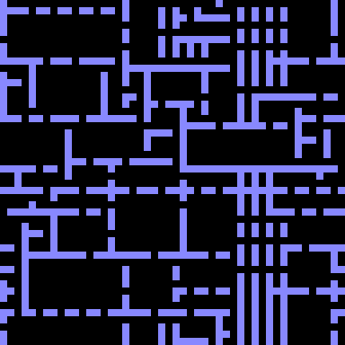
The gaps between the tiles in the input were transparent, and in the output they are black, which alerted me to the fact that the wfc_image crate currently throws away transparency.
Broken Probability Distribution
I was originally planning to use this image as an example:

I expected to see a roughly equal number of upwards sloping tiles and downwards sloping tiles (as the input image is wrapped when sampling tiles):
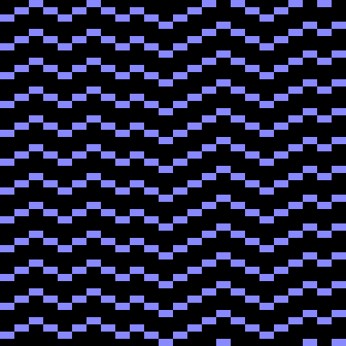
But instead, the output was almost entirely made up of upwards sloping tiles:
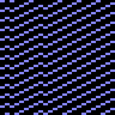
After much debugging, I traced the problem to a bug in my implementation of randomly choosing from a probability distribution:
commit ede0ea4ed4560bdcf85b4dda989937484bfec21e
Author: Stephen Sherratt <sfsherratt@gmail.com>
Date:   Sun Feb 10 21:37:59 2019 +0000

    Fix bug in probability distribution

diff --git a/wfc/src/wfc.rs b/wfc/src/wfc.rs
index 21ac889..03e6cc7 100644
--- a/wfc/src/wfc.rs
+++ b/wfc/src/wfc.rs
@@ -475,7 +475,7 @@ impl WaveCell {
         for (pattern_id, pattern_stats) in
             self.weighted_compatible_stats_enumerate(global_stats)
         {
-            if remaining > pattern_stats.weight() {
+            if remaining >= pattern_stats.weight() {
                 remaining -= pattern_stats.weight();
             } else {
                 assert!(global_stats.pattern_stats(pattern_id).is_some());