Visible Area Detection with Recursive Shadowcast
Most games employ some form of visible area detection to simulate the fact that opaque objects obscure one’s view of whatever is behind them. Recursive Shadowcast is one of a handful of algorithms that compute visible area in worlds represented by 2D grids. This makes it suitable for use in roguelikes. This post will explain the recursive shadowcast algorithm.
Visible Area Detection in a 2D Grid
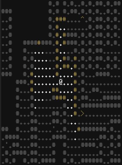
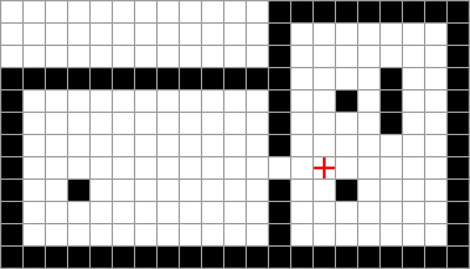
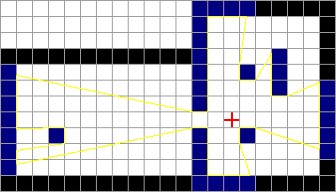
Before diving into the details, let’s get a feel for 2D grid-based visible area detection. Below is an environment that will be used throughout this post. White cells are empty and black cells are opaque walls. The scene is viewed from the cell containing the red cross.
The yellow-shaded area in the image below is visible from the centre of the observer’s cell.
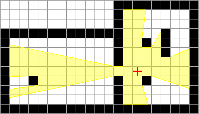
Note that some cells are partially inside the visible area. To simplify explanations, these cells will be considered to be completely visible.
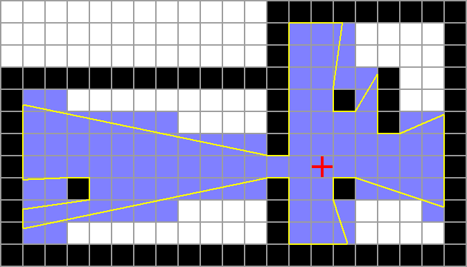
The visible floor cells are shown below.
If at least one edge of a wall cell is visible, it is considered visible. Visible wall cells are shown below.
Recursive Shadowcast
Recursive Shadowcast takes the following input:
- a 2D grid of cells, where each cell is either transparent or opaque
- a coordinate of a cell in this grid from which the scene is viewed
It identifies which cells in the grid are visible when viewed from the specified position.
Octants
Recursive shadowcast considers the space to be made up of 8 octants, centred at the observer. Each coloured segment in the image below is a single octant. The visible area is computed independently on each octant.
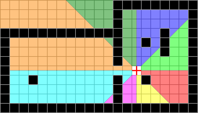
If a cell lies on the border of 2 octants, it is considered to be in both. This implies that some cells are in 2 octants. It would be trivial to keep track of which cells have been visited, and thus prevent visiting the same cell twice while processing two different octants if necessary.
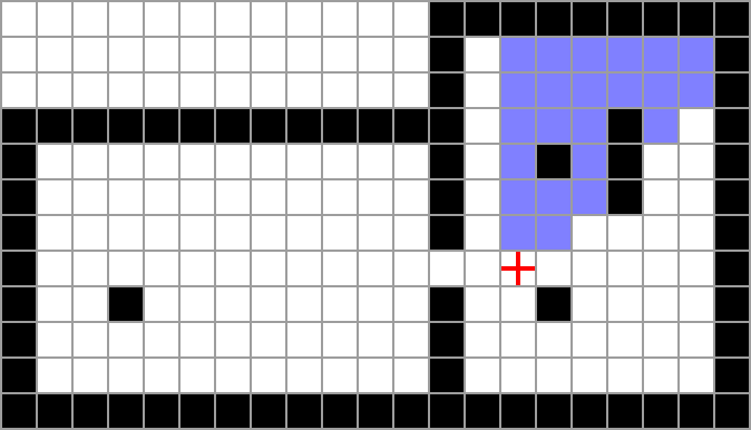
To clarify the point above, shaded in blue below are all the cells in a single octant.
Note also that the cell containing the observer isn’t part of any octant. Generally, the cell containing the observer is always visible, regardless of the opacity of the cells around them.
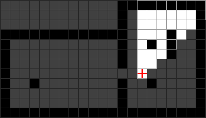
Example Octant
The simplest way to explain this algorithm is to jump right in with an example. We’ll first consider this octant.
As we compute the visible area in this octant, we’ll be keeping track of a few variables:
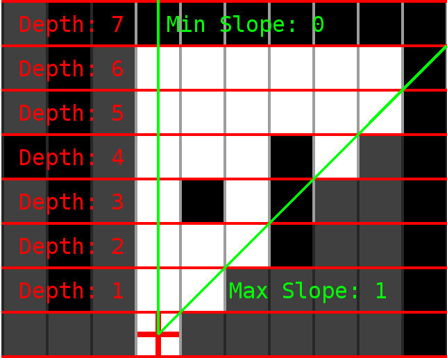
- depth is the vertical distance of a cell (or row of cells) from the eye. Computation always starts with depth = 1.
- min slope is the gradient of the left-most edge of our vision (within this octant)
- max slope is the gradient of the right-most edge of our vision (within this octant)
For this octant, gradient values are ratios dx/dy relative to the eye’s position. That is, multiplying a gradient value by some distance above the eye, will give a corresponding distance to the right of the eye on the slope defined by the gradient. Thus, as in the image below, a gradient of 0 defines a line going straight up, and a gradient of 1 defines a line at 45 degrees up and to the right.
It’s important to point out that the eye is considered to be in the centre of its cell. That is, if the eye is in cell at coordinates (2, 3), the actual absolute position of the eye would be (2.5, 3.5) (assuming (0, 0) is the coordinate of the top-left corner of the grid).
We’ll scan the current depth from west to east. Each cell that is visited is considered to be visible. If an opaque cell is encountered, recurse, incrementing the depth, and adjusting the min and max slope such that the opaque cell obscures vision at the next depth level. This process is documented more concretely in the following pseudocode.
computeVisibleArea(current_depth, min_slope, max_slope) {

  first = true;
  previous_cell = null;

  for each cell "current_cell" at depth "current_depth"
                        between "min_slope" and "max_slope"
                        from west to east {

    mark current_cell as visible;

    if not first {

      if current_cell is opaque and previous_cell is transparent {

        # first opaque cell after at least one transparent cell
A:      next_max_slope = gradient of line passing through eye and
                            northwest corner of "current_cell";

        computeVisibleArea(current_depth+1, min_slope, next_max_slope);
      }

      if current_cell is transparent and previous_cell is opaque {

        # first transparent cell after at least one opaque cell
B:      min_slope =  gradient of line passing through eye and
                            southwest corner of "current_cell";

      }

    } else {
      first = false;
    }

    previous_cell = current_cell;
  }

  if previous_cell is transparent {

    # see through last group of transparent cells in row
C:  computeVisibleArea(current_depth+1, min_slope, max_slope);
  }

}
The interesting parts of the code are labelled with A, B and C. We’ll visit each case as we work through the example octant.
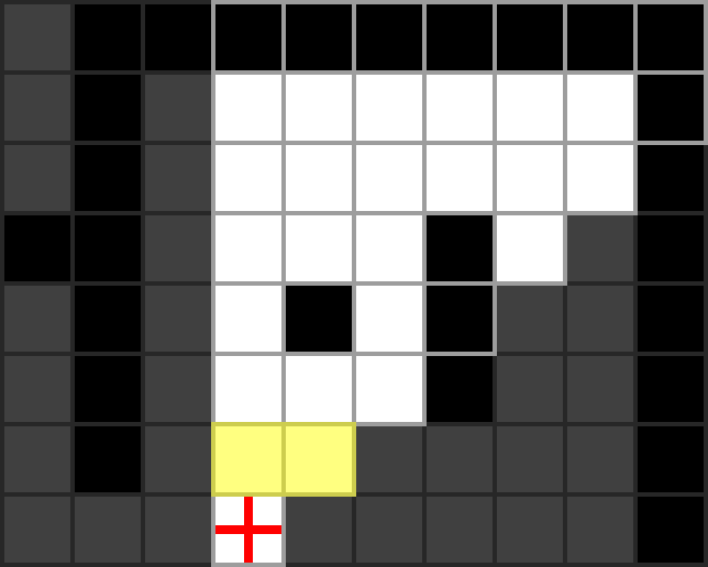
Initially, the function is called with arguments: computeVisibleArea(1, 0, 1).
The scan at depth 1 (below) is simple as there are no opaque cells. The only case in the
code above that we encounter here is case C. After scanning each cell,
previous_cell refers to the right-most cell at this depth (since we scan from
west to east), which is transparent. Thus we recurse to depth 2, leaving the
min_slope and max_slope arguments unchanged as they are passed to the
recursive call.
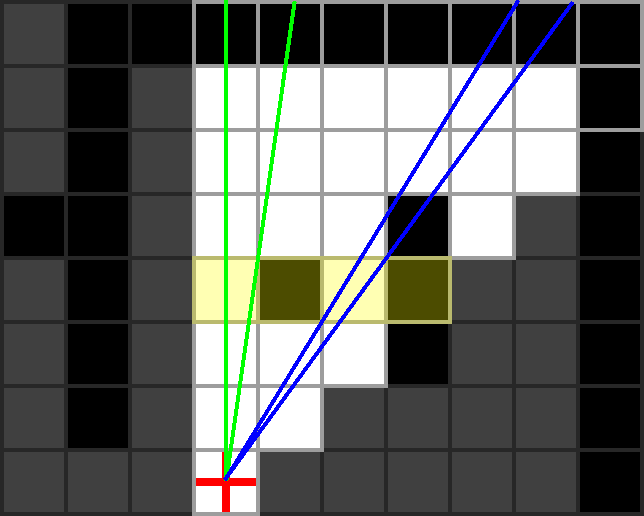
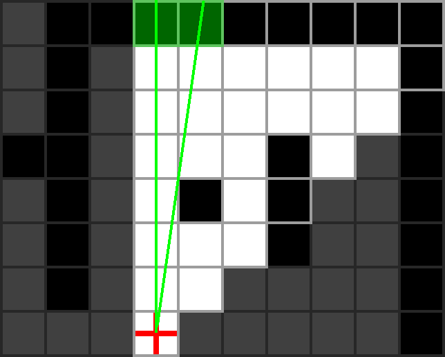
Depth 2 is the same as depth 1 in that none of the cells are visible, so we will skip it and move straight on to depth 3, which is much more interesting. Unlike the previous depths, there are 2 recursive calls made on depth 3 (represented by the green and blue pairs of lines in the image below).
Moving west to east, when the second cell at this depth is visited, the code
above will hit case A, as an opaque cell is visited after a transparent cell.
The value of next_max_slope for this case is the gradient of the right-most
green line. Note that this line passes through the eye and the northwest corner
of the second cell. The left-most green line has a gradient of min_slope (0 in this
case) which was passed to this function as an argument. These two gradients are
passed to the recursive call, along with an incremented depth (4).
The third cell visited at depth 3 causes the code to hit case B, as a
transparent cell is visited after an opaque cell. In this case, no recursive
call is made, but the value of min_slope is adjusted to be the gradient of the
left-most blue line. Note that this line passes through the eye and the
southwest corner of the third cell.
Finally, the fourth cell at this depth causes the code to hit case A again,
meaning a new next_max_gradient is calculated (the right-most blue line) and
the code makes a second recursive call for this depth. Note again, that the
right-most blue line passes through the eye, and the northwest corner of the
opaque cell.
Unlike the previous depths, case C is not reached, as the last cell visited at this depth is not transparent.
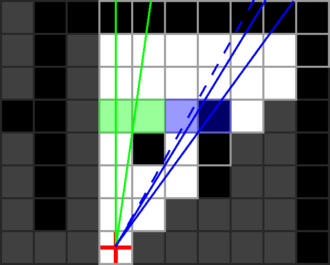
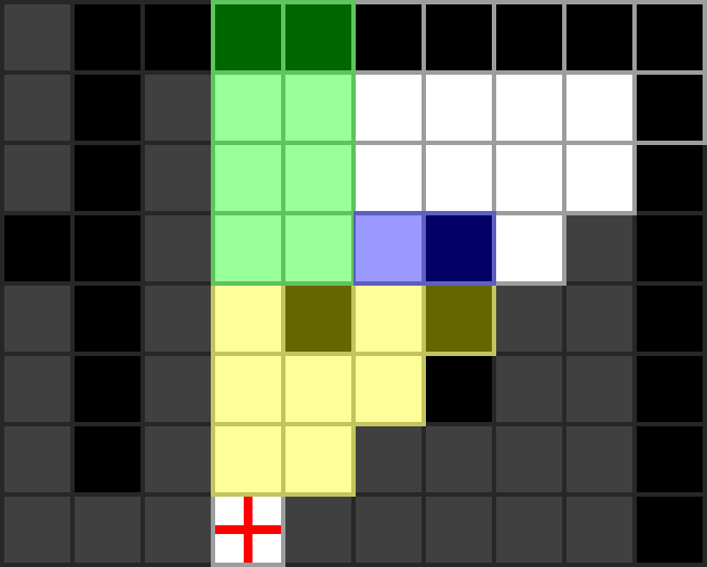
Depth 4 is reached by 2 separate recursive calls. It’s important to note here
that all cells even partially inside the area between a pair of coloured lines
be considered in the corresponding scan (hence the shading in the image below).
The green instance is simple as there are no opaque cells. The blue instance
will hit case A, though note that next_max_slope (the dotted line below) will
be less than (ie. to the left of) min_slope. This means no cells could be
between then. Thus the blue instance stops here.
The final case to consider in this example is the very last recursion of the green instance. Shown below, this case is unique as no cells in the scan are transparent. Stepping through the code, we see that each cell is marked as visible (as normal), but neither case A, nor C are hit, meaning no recursion is made, and execution stops.
The shaded cells in the image below are all the cells marked as visible in this octant using recursive shadowcast.
Generalizing to all Octants
The solution presented in the previous section is specific to the example octant. The following features of the algorithm are specific to that octant:
- As
depthincreases, we move north. - We scan west to east.
min_slopestarts at 0.max_slopestarts at 1.- When visiting an opaque cell after a transparent cell, the northwest corner of
the opaque cell is used to find
next_max_slopefor the recursive call. - When visiting a transparent cell after an opaque cell, the southwest corner of the transparent cell
is used to find the new value of
min_slope.
Let’s see how these characteristics change in different octants. Note that this is just one of many possible ways to represent the differences between octants. These are in no way canonical.
The image below shows the direction to move in the grid as the depth
increases. In the north-most octants we move north, in the east-most we move
east, and so on.
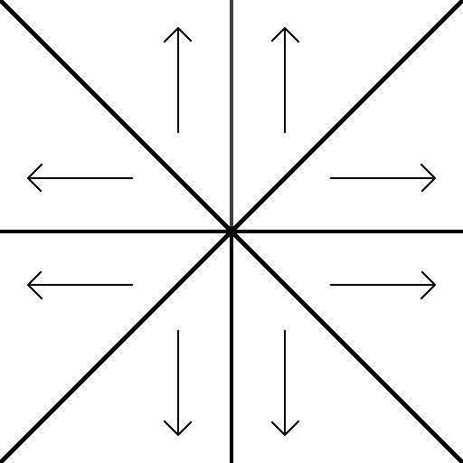
Depth Direction
Closely relate to this is the scan direction. It can be derived from the depth direction: if you stand facing the depth direction for an octant, the scan direction for that octant will be from your left, to your right.
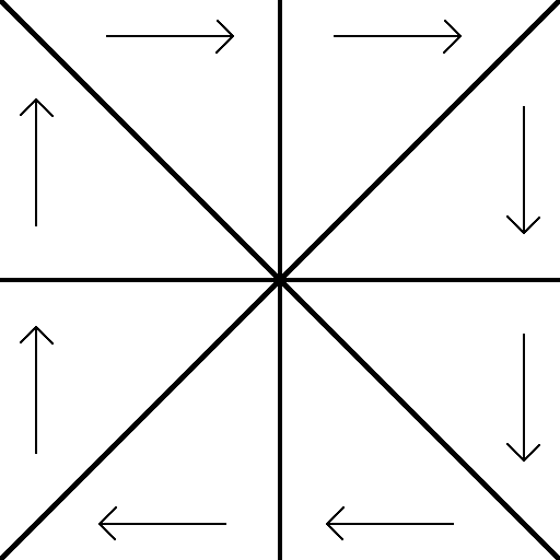
Scan Direction
Tied into the above two characteristics is the initial values of min_slope and
max_slope. For any pair of octants sharing a common depth direction (or scan
direction), if you stand facing the depth direction, the octant to your left
would have slopes ranging from -1 to 0, and the octant to your right from 0 to 1.
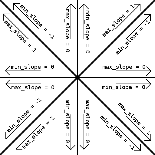
Initial values for min_slope and
max_slope
When scanning cells in the octant’s scan direction, if an opaque cell is visited after
a transparent cell, we compute a new maximum depth (next_max_depth) to pass to a recursive call
based on one of the corners of the opaque cell. In the previous example, that
was the northwest corner.
Similarly, when visiting a transparent cell after an opaque cell, the current min_slope is adjusted
based on one of its corners. This is the southwest corner in the example.
Which corners to choose in this cases is octant-dependent, and is shown in the
diagram below.
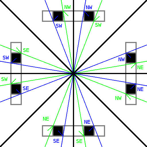
Cell corners to use for finding slopes
Many of these characteristics are related in some way, and knowledge of some can be used to derive others. Despite this, for simplicity, when computing the visible area for a given octant, let’s just pass all the characteristics as arguments:
computeVisibleArea(current_depth, min_slope, max_slope,
                   depth_direction, scan_direction,
                   opaque_corner, transparent_corner) {

  first = true;
  previous_cell = null;

  for each cell "current_cell" at depth "current_depth"
                        between "min_slope" and "max_slope"
                        in "scan_direction" {

    mark current_cell as visible;

    if not first {

      if current_cell is opaque and previous_cell is transparent {

        # first opaque cell after at least one transparent cell
A:      next_max_slope = gradient of line passing through eye and
                          "opaque_corner" corner of "current_cell";

        computeVisibleArea(current_depth+1, min_slope, next_max_slope,
                           depth_direction, scan_direction,
                           opaque_corner, transparent_corner);
      }

      if current_cell is transparent and previous_cell is opaque {

        # first transparent cell after at least one opaque cell
B:      min_slope =  gradient of line passing through eye and
                        "transparent_corner" corner of "current_cell";

      }

    } else {
      first = false;
    }

    previous_cell = current_cell;
  }

  if previous_cell is transparent {

    # see through last group of transparent cells in row
C:  computeVisibleArea(current_depth+1, min_slope, max_slope,
                       depth_direction, scan_direction,
                       opaque_corner, transparent_corner);
  }
}
Iterative Shadowcast
Passing these characteristics as arguments to the recursive function is repetitive, since within an octant they never change, and recursive calls never go between octants. An alternative way of structuring this function that removes the need to pass them around, is to replace the recursion with iteration.
We’ll need a data structure representing state once represented by a recursive
call. The arguments that could change with each recursive call are depth,
min_slope and max_slope. Thus, our structure will look like:
class StackFrame {
  depth;
  min_slope;
  max_slope;

  constructor(depth, min_slope, max_slope) {
    this.depth = depth;
    this.min_slope = min_slope;
    this.max_slope = max_slope;
  }
}
Using this, and an assumed Stack data structure, the code becomes:
computeVisibleArea(initial_min_slope, initial_max_slope,
                   depth_direction, scan_direction,
                   opaque_corner, transparent_corner) {

  # Make this a global variable or equivalent to remove the
  # overhead of constructing it each time this is called.
  stack = new Stack();

  initial_frame = new StackFrame(1, initial_min_slope,
                                    initial_max_slope);

  stack.push(initial_frame);

  while stack is not empty {

    current_frame = stack.pop();
    current_depth = current_frame.depth;
    min_slope = current_frame.min_slope;
    max_slope = current_frame.max_slope;

    first = true;
    previous_cell = null;

    for each cell "current_cell" at depth "current_depth"
                          between "min_slope" and "max_slope"
                          in "scan_direction" {

      mark current_cell as visible;

      if not first {

        if current_cell is opaque and
            previous_cell is transparent {

          # opaque cell after at a transparent cell
A:        next_max_slope = gradient of line passing through eye and
                            "opaque_corner" corner of "current_cell";

          next_frame = new StackFrame(current_depth+1,
                                      min_slope, next_max_slope);

          stack.push(next_frame);
        }

        if current_cell is transparent
            and previous_cell is opaque {

          # transparent cell after at opaque cell
B:        min_slope =  gradient of line passing through eye and
                        "transparent_corner" corner of "current_cell";

        }

      } else {
        first = false;
      }

      previous_cell = current_cell;
    }

    if previous_cell is transparent {

      # see through last group of transparent cells in row
C:    next_frame = new StackFrame(current_depth+1,
                                  min_slope, max_slope);
      stack.push(next_frame);
    }
  }
}
All the recursive calls were replaced with creating a new object with the information that would have been passed to the recursive call, and pushing it onto a stack. Keep iterating until the stack is empty, removing the most recently pushed data each time. This will change the order in which cells are visited. In the recursive version, when a recursive call was made, the current scan would be put on hold while the scan at the next depth was performed, which may itself have made a recursive call, etc, etc. In the iterative version, while doing a scan, any would-be recursive calls have their arguments pushed onto a stack. Once the scan is finished, the same set of next-depth scans will occur as in the recursive version, but in the reverse order. Take some time to convince yourself that despite the new order, the same cells are visited, and thus the same cells are classified as visible.
Another minor change is the removal of the depth argument. This is no longer
needed because the function’s arguments are now just initial values, and the
depth always starts at 1.
Putting it all together, we need to call computeVisibleArea once for each
octant, giving it the relevant arguments for that octant. The following function
does this, starting with the octant in the example above, going around
clockwise.
computeTotalVisibleArea() {
  computeVisibleArea(0, 1,  North, East, NorthWest, SouthWest);
  computeVisibleArea(-1, 0, East, South, NorthWest, NorthEast);
  computeVisibleArea(0, 1,  East, South, NorthEast, NorthWest);
  computeVisibleArea(-1, 0, South, West, NorthEast, SouthEast);
  computeVisibleArea(0, 1,  South, West, SouthEast, NorthEast);
  computeVisibleArea(-1, 0, West, North, SouthEast, SouthWest);
  computeVisibleArea(0, 1,  West, North, SouthWest, SouthEast);
  computeVisibleArea(-1, 0, North, East, SouthWest, NorthWest);
}